Exact Wavefunctions with Deep Neural Networks

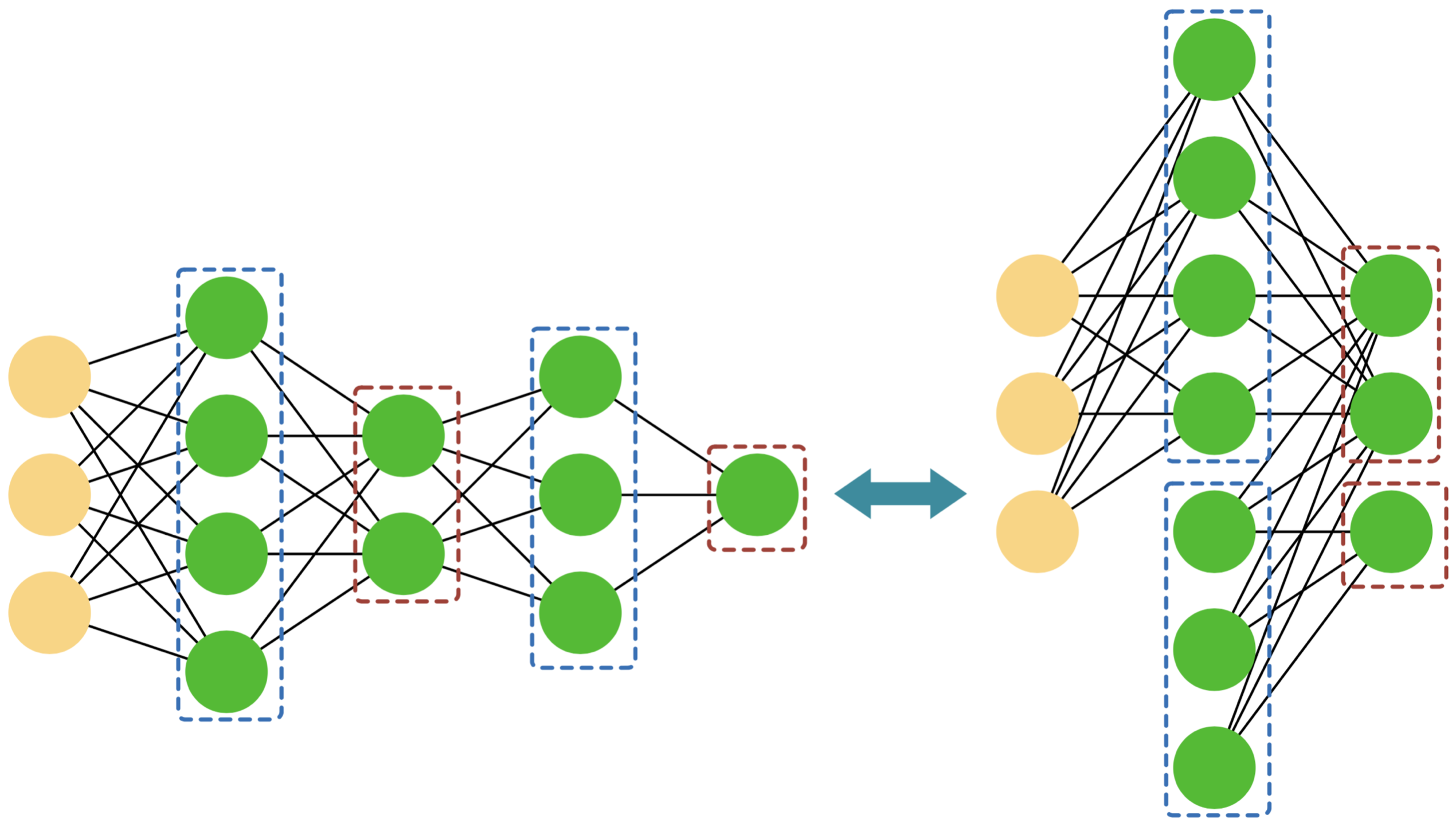
The state of a spin-1/2 system in the \(\sigma^z\)-basis, when encoded by a DBM, can therefore be written as\[\Psi_{\mathcal W}(\sigma^z)=\sum_{\{h,d\}} \exp\bigg[\sum_i \big(a_i\sigma_i^z + b_ih_i +b_i'd_i\big)\\
+\sum_{ij}\big( \sigma_i^z W_{ij}h_j + h_iW_{ij}' d_j \big)\bigg]\]
In this expression,  \(h\) and \(d\)  denote the spins of the first and second hidden layer, respectively, which come with their individual weights and biases. At first sight, we run into a problem when we want to optimize the parameters \(\mathcal{W}=(W,b,W',b')\) of a DBM so as to best approximate a given ground state: Remember that for a RBM, one can evaluate the summation over all hidden spins, thus determining the form of the corresponding wavefunction analytically. This is however not anymore possible for a DBM, making the task of tracing back changes in the parameters to changes in the energy costly, and therefore also the task of training a DBM.

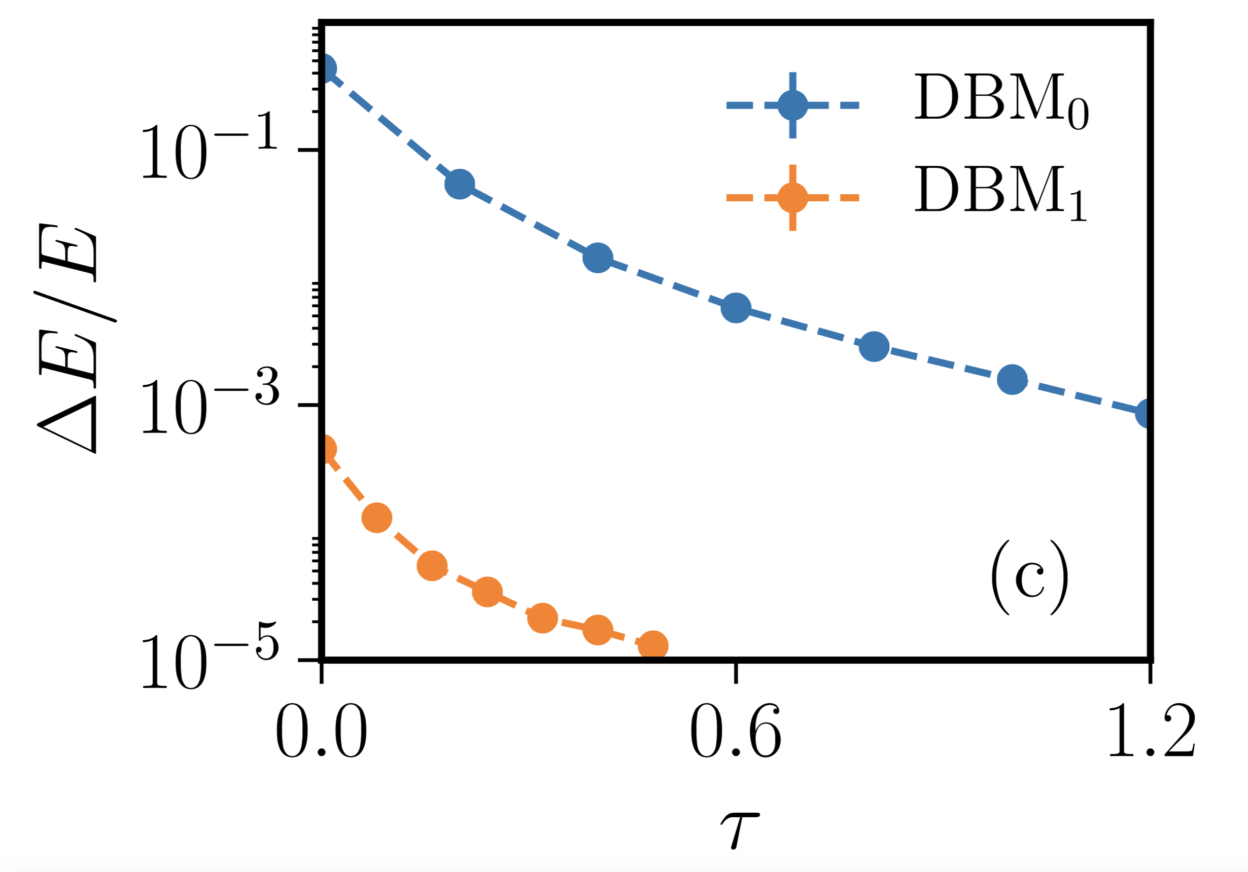
Carleo, Nomura and Imada [3] show how to avoid this problem: They provide a prescription to efficiently optimize the parameters of a DBM for two paradigmatic one-dimensional spin-1/2 models of many-body physics, the transverse-field Ising model and the Heisenberg model. Their idea is to perform an exact imaginary-time evolution in the parameter space of DBMs instead of just employing them as variational wavefunctions. Remember that any ground state of a gapped Hamiltonian \(H\) can be written as the infinite-time limit of the imaginary-time evolved state \(|\Psi(\tau)\rangle = e^{-\tau H}|\Psi(0)\rangle\), where \(|\Psi(0)\rangle \) denotes an arbitrary state that has non-zero overlap with the true ground state. When we make the ansatz \[\langle \sigma_1^z\cdots \sigma_N^z|\Psi(\tau)\rangle = \Psi_{\mathcal W}(\sigma^z)\] we can map this time evolution to an evolution of the DBM parameters \({\mathcal W}(\tau)\). Ref. [3] then proceeds to show how such an exact mapping can be achieved in the case of the two models mentioned above. This algorithm therefore allows to encode the eigenstates of the respective model faithfully at every step of the imaginary-time evolution, without the need for a variational optimization of the DBM parameters. To achieve this, it turns out to be necessary to add a number of hidden neurons to the DBM at every timestep that is proportional to the system size. The total number of DBM parameters is therefore linear in the elapsed imaginary time, as well as in the system size. Note that the only discrepancy of the so obtained DBM state with respect to the true ground state comes from the fact that \(\tau\) is finite.

There are a few open questions that are left unanswered by Ref. [3]. While the authors provide an efficient algorithm to arrive at the ground states of the one-dimensional transverse-field Ising and Heisenberg models, it remains unclear whether we can find an exact representation of the imaginary-time evolution in terms of DBM parameters for all physically relevant models, especially in higher dimensions. There is also no attempt made of a comparison of this method with the established matrix-product state algorithms that perform imaginary-time evolution efficiently in one dimension. It thus remains an open question whether the DBM based imaginary-time evolution presented here will contribute to the understanding of those problems of many-body physics that have so far also eluded the conventional methods of the field.